Confidence, thresholds and calibration
作者: Jakub Rusinowski · 最后更新:
A decision model's probabilities are only useful if a 0.9 is right about 90% of the time. That property is called calibration, and you have to measure it on your own data — Ollama's confidence field does not measure it. Label 100–300 real examples, run them through the model, and set three bands: accept automatically, send to a bigger model or a human, and abstain. This page shows how, with a script you can run tonight.
Three different numbers people call "confidence"
| Number | Where it comes from | What it tells you |
|---|---|---|
probabilities | Every choice and score answer; noul is the probability of true | The model's belief spread across your options |
confidence (Ollama) | Ollama computes 1 − H(p) / ln(N) — one minus the normalised entropy of the probabilities | How peaked the distribution is. 0 = all options equally likely; near 1 = one option dominates |
| Calibration | You measure it: compare stated probability with how often the model was actually right | Whether you can trust the probabilities at face value |
Ollama's API reference is explicit that confidence is "not calibrated correctness", and its decision guide adds that "a higher value does not guarantee the answer is correct." TypeSafe markets its hosted Jev as calibrated and trains for it with RLCD — but that claim is about Jev, not about the open models you run locally. Some open models publish calibration numbers on their cards; treat those as a starting point, not a guarantee on your data.
A worked example of why peakedness isn't correctness: ask "Is this date before 2024?" about "03/04/2025". A model can say noul: 0.02 — very peaked, very confident — and be reading the date as text rather than comparing it. TypeSafe's own list of Jev's failure modes includes dates, numbers, double negatives and instructions hidden inside the state. Smaller open models share those weaknesses, usually more strongly.
What good calibration looks like
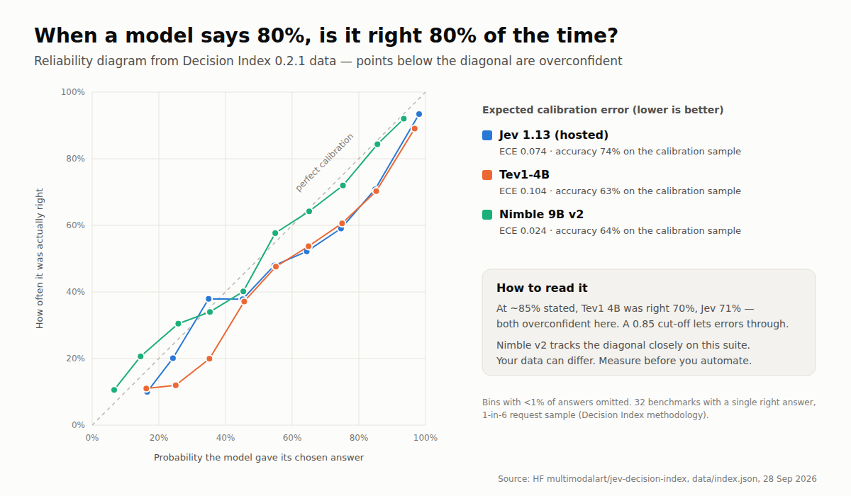
Group your test answers into bins by the probability of the chosen option (0.5–0.6, 0.6–0.7, …). In each bin, compute how often the model was right. A calibrated model's accuracy in the 0.8–0.9 bin is about 0.85. An overconfident model says 0.9 and is right 70% of the time — the common failure, and the dangerous one, because your code will auto-accept those answers.
The single-number summary is expected calibration error (ECE): the weighted average gap between stated probability and actual accuracy across bins. Lower is better. On the community Decision Index (snapshot 28 September 2026), Jev 1.13 has an ECE of 0.074; open models range from 0.014 (Jebadiah 27B) to above 0.5. A low ECE on a public benchmark is encouraging; it doesn't transfer automatically to your tickets, your policies, your language.
Accuracy is not calibration
Accuracy counts how often the top answer is right. Calibration asks whether the probabilities mean what they say. A model can be accurate and badly calibrated at once, and a threshold depends only on the second. Two models with the same 90% accuracy can need completely different thresholds: one says 0.9 when it is right and 0.6 when it is wrong, the other says 0.97 either way. You can automate the first. The second gives you nothing to set a threshold on.
Four numbers, in plain words:
| Metric | What it measures | How to read it |
|---|---|---|
| Accuracy | The share of answers whose top option is correct | Ignores the probabilities entirely |
| ECE (expected calibration error) | Bin answers by stated probability; in each bin, take the gap between average stated probability and the share actually right; average the gaps, weighted by bin size | An ECE of 0.05 means the stated probabilities are off by about five points on average. It depends on the number of bins, so report that number with it |
| NLL (negative log-likelihood, or log loss) | Minus the log of the probability the model gave the correct answer, averaged | Punishes confident mistakes hardest: one wrong answer at 0.99 costs more than many wrong answers at 0.6 |
| Brier score | The mean squared gap between the stated probability and what happened (1 if right, 0 if wrong) | Lower is better. It rewards being both calibrated and decisive, so a model that always says 0.5 scores poorly even when it is never overconfident |
Report all four from the same run. ECE alone can look excellent for a model that hedges everything near its own accuracy; NLL and Brier expose that. Accuracy alone tells you nothing about where to put a threshold.
Reading the reliability diagram above. The horizontal axis is the probability the model stated; the vertical axis is how often it was right in that bin. Points on the diagonal are calibrated. Points below it are overconfident (it said 0.9, it was right 70% of the time), which is the dangerous side, because those answers clear your threshold. Points above it are underconfident, which only costs you coverage. Always print the number of answers in each bin beside the diagram: a bin with eight answers in it is noise, however far it sits from the line.
Published ECE values are illustrations, not predictions. The same checkpoint scores differently on different suites, which is exactly the point:
| Model | ECE | Measured on | Who measured it | Source |
|---|---|---|---|---|
| Bosun v3.1 0.6B | 0.1419 | Decision Index 0.2.1 | Community Decision Index (not by the model's authors) | — |
| Bosun v3.1 0.6B | 0.0588 | DecisionBench 1.0 (Hanno Labs): Applied suite (22,700 rows) | Benchmark built by the same team that built this model | source ↗ |
| Bosun v3.1 0.6B | 0.0659 | DecisionBench 1.0 (Hanno Labs): All rows, including the 1,200-row reasoning track (23,900 rows) | Benchmark built by the same team that built this model | source ↗ |
| Bosun v3.1 1.7B | 0.1302 | Decision Index 0.2.1 | Community Decision Index (not by the model's authors) | — |
| Bosun v3.1 1.7B | 0.0397 | DecisionBench 1.0 (Hanno Labs): Applied suite (22,700 rows) | Benchmark built by the same team that built this model | source ↗ |
| Bosun v3.1 1.7B | 0.0497 | DecisionBench 1.0 (Hanno Labs): All rows, including the 1,200-row reasoning track (23,900 rows) | Benchmark built by the same team that built this model | source ↗ |
| OpenDecider-nano | 0.092 | 200 general decisions (BANKING77, BoolQ, Yelp, ChaosNLI): 200 decisions | Run by the authors on a public third-party harness | source ↗ |
| OpenDecider-small | 0.087 | 200 general decisions (BANKING77, BoolQ, Yelp, ChaosNLI): 200 decisions | Run by the authors on a public third-party harness | source ↗ |
Lower is better. The same model gets a different ECE on each suite, because calibration is a property of a model on a distribution. Compare ECE only within one suite; never across rows from different suites.
Compare the Bosun rows: the ECE its own team measured on DecisionBench is far lower than the one the community Decision Index measured on its own questions. Neither number is wrong. Calibration belongs to a model on a distribution, and yours is a third distribution.
From calibration to an operating point: the risk–coverage curve
Sort your labelled answers by the probability of the chosen option. For each candidate threshold, coverage is the share of answers at or above it (the ones you would automate), and selective risk is the error rate among those answers. Plot risk against coverage. The curve answers the only question the business cares about: at an error rate I can live with, how much of the traffic can I automate? The coverage_curve() function in the script below prints exactly these pairs.
Pick the accept threshold where selective risk meets your tolerance. Everything below it goes to the escalate band, and only the answers so uncertain that even a second opinion would be guessing go to abstain (see three bands, not one threshold). Re-draw the curve whenever the model, its quantisation or the question wording changes.
Per-task temperature scaling
If the diagram shows a model consistently overconfident on one question, you can fix that question without retraining. Temperature scaling divides the log-probabilities by one number T, fitted on labelled data, and renormalises. T > 1 softens overconfident answers, T < 1 sharpens timid ones, and because every option is scaled the same way, the top answer never changes. Only the probabilities move, so accuracy stays put while ECE and NLL improve.
Fit T per question type, per task. A routing choice and a refund noul are miscalibrated in different directions, and one global T can make one of them worse. Hold out part of your labelled set: fit T on one half, check ECE on the other.
# fit_temperature.py — one temperature per question, fitted by minimising NLL
# rows: list of (probabilities: dict[str, float], label: str) from your eval run
import math

def scaled(probs, t):
    logits = {k: math.log(max(p, 1e-12)) / t for k, p in probs.items()}
    z = sum(math.exp(v) for v in logits.values())
    return {k: math.exp(v) / z for k, v in logits.items()}

def nll(rows, t):
    return -sum(math.log(max(scaled(p, t)[y], 1e-12)) for p, y in rows) / len(rows)

def fit_temperature(rows):
    grid = [x / 100 for x in range(25, 501)]          # T from 0.25 to 5.00
    return min(grid, key=lambda t: nll(rows, t))

# t = fit_temperature(train_rows); then apply scaled(probs, t) before your thresholds
Apply the fitted T in your own code, before the thresholds. Re-fit it whenever you change model version, quantisation or runtime, for the same reason you re-draw the risk–coverage curve.
Sources, checked 2026-10-14: Guo et al. 2017, calibration of neural networks and temperature scaling · Geifman & El-Yaniv 2017, selective classification and risk–coverage · scikit-learn: log loss (NLL) · scikit-learn: Brier score · scikit-learn: probability calibration and calibration curves.
Measure it on your data — the 30-minute version
- Collect 100–300 real examples for one question. Real, not invented — invented examples are easier than production.
- Label them yourself (or two people, and discard disagreements).
- Run them through the model with the exact question wording you'll use in production.
- Compute accuracy, ECE and the accuracy-vs-coverage curve with the script below.
- Pick thresholds from the curve, then re-check on a fresh batch a month later.
Save your examples as JSON Lines, one decision per line:
{"state": "I was charged twice. Please refund the extra payment.", "label": "billing"}
{"state": "The app crashes when I open settings.", "label": "technical"}
Then run this against your local Ollama. It needs only requests:
# eval_decisions.py — measure accuracy and calibration of one choice question
# Usage: python eval_decisions.py examples.jsonl nimble
import json, sys, requests

URL = "http://localhost:11434/v1/systemone"
QUESTION = {
    "type": "choice",
    "instructions": "Which team should handle this ticket?",
    "criteria": {
        "billing": "Payments and refunds",
        "technical": "Bugs and integrations",
        "other": "None of the above",
    },
}

def run(path, model):
    rows = []
    with open(path, encoding="utf-8") as f:
        for line in f:
            ex = json.loads(line)
            r = requests.post(URL, json={
                "model": model,
                "state": ex["state"],
                "questions": {"q": QUESTION},
                "keep_alive": "10m",
            }, timeout=120)
            r.raise_for_status()
            a = r.json()["answers"]["q"]
            p = a["probabilities"][a["choice"]]
            rows.append((p, a["choice"] == ex["label"]))
    return rows

def ece(rows, bins=10):
    total, err = len(rows), 0.0
    for b in range(bins):
        lo, hi = b / bins, (b + 1) / bins
        in_bin = [(p, ok) for p, ok in rows if lo < p <= hi or (b == 0 and p == 0)]
        if not in_bin:
            continue
        conf = sum(p for p, _ in in_bin) / len(in_bin)
        acc = sum(ok for _, ok in in_bin) / len(in_bin)
        err += len(in_bin) / total * abs(conf - acc)
    return err

def coverage_curve(rows, thresholds=(0.5, 0.6, 0.7, 0.8, 0.9, 0.95)):
    for t in thresholds:
        kept = [ok for p, ok in rows if p >= t]
        cov = len(kept) / len(rows)
        acc = sum(kept) / len(kept) if kept else float("nan")
        print(f"accept if p >= {t:.2f}: covers {cov:6.1%} of traffic, accuracy {acc:6.1%}")

if __name__ == "__main__":
    rows = run(sys.argv[1], sys.argv[2] if len(sys.argv) > 2 else "nimble")
    acc = sum(ok for _, ok in rows) / len(rows)
    print(f"n={len(rows)}  accuracy={acc:.1%}  ECE={ece(rows):.3f}")
    coverage_curve(rows)
The output reads like this (illustrative numbers, not a measurement):
n=200  accuracy=86.0%  ECE=0.061
accept if p >= 0.50: covers 100.0% of traffic, accuracy  86.0%
accept if p >= 0.70: covers  88.5% of traffic, accuracy  92.1%
accept if p >= 0.90: covers  71.0% of traffic, accuracy  97.2%
accept if p >= 0.95: covers  58.5% of traffic, accuracy  98.3%
That last table is the whole decision: "if I auto-accept everything above 0.9, I handle 71% of tickets automatically at 97% accuracy, and a human sees the other 29%." Whether 97% is good enough is a business question, not a model question.
Set three bands, not one threshold
p ≥ accept_threshold          → act automatically
review ≤ p < accept_threshold → escalate: bigger model, second opinion, or a human
p < review → abstain: don't guess; fall back to the safe default- Per question, per type. A threshold tuned on a
nouldoesn't carry over to achoice, even on the same topic — TypeSafe documents that a model's answer to a question and to its reworded opposite don't necessarily sum to 1. - Escalate cheaply. Run
tev1first; send only the uncertain band tonimbleor an open 27B reproduction; send what's still uncertain to a human. Most traffic never touches the big model. - Use margin for
choice. The gap between the top two probabilities is often a better escalation signal than the top probability alone, especially with many options. - Read
scorecarefully.scoreis a weighted average of level indices, so a 0.9 on a three-level scale can come from a model split between levels 0 and 2 — look atprobabilitiesbefore acting on it. Score is also the weakest primitive: Nimble scores 54.6% on it versus about 80% on choice and yes/no in Bespoke's public benchmark.
Things that change probabilities without changing answers
- Temperature. Some model repos ship a calibration temperature (Bespoke's original Nimble checkpoint used T = 2.179, its September checkpoint T = 1.0; Decider applies a separate temperature per answer type). Temperature reshapes the probabilities but never changes which option is highest. Re-tune your thresholds whenever you switch model version or runtime.
- Quantisation. A Q4 build can pick the same answers as BF16 and still shift the probabilities. JevK5's card reports its Q4_K_M build matching BF16 answers on 221 of 231 public items — close, not identical. Measure on the build you'll run.
- Wording. Option descriptions carry the meaning. Question names are labels for your code — Decider, for one, never shows them to the model. If you leave an option's description
null, Ollama uses the key itself as the option text, so"billing": nullis weaker than"billing": "Payments, invoices and refunds".
Frequently asked questions
Is a high confidence in Ollama a good sign?
It means the model strongly favours one option. That's necessary for a trustworthy answer but not sufficient: a model can be confidently wrong. Measure calibration on your data before you use it as an automation threshold.
How many examples do I need?
100 labelled examples gives you a rough accuracy number; 300 or more lets you see calibration per bin. Add more for rare but costly cases — refund fraud, safety violations — because an overall accuracy number hides them.
Should I trust the ECE numbers on model cards and leaderboards?
They're useful for comparing models on the same benchmark. They don't predict calibration on your distribution. A model trained on customer-support tickets can be well calibrated there and overconfident on legal clauses. The evaluation guide shows how to weigh each kind of published score and test the model on 200 of your own rows.
Should I report ECE, NLL or the Brier score?
All three, from the same run, plus accuracy. ECE is the easiest to explain but can look good for a model that hedges everything; NLL and the Brier score catch that. For setting a threshold, the risk–coverage curve is what you actually read.
Can I recalibrate a model myself?
Yes. The simplest method is temperature scaling: fit one number on your labelled set that rescales the probabilities to match observed accuracy. Several open decision models ship exactly that as a config value. It improves calibration without changing any answer. --- Definitions from docs.ollama.com/api/systemone and /capabilities/decision; failure modes from TypeSafe's jev-1.13 model jaggedness page; model figures from the Bespoke Nimble README and the Decision Index 0.2.1 data. Read 30 September 2026.
Keep going
- Decision models (Jev-style System One): run them locally
- Run Jev-style decision models locally with Ollama (Nimble, Tev1)
- Open Jev reproductions beyond Ollama: Winnow, Decider, JevK5, AutoJev, Laya
- Decision models on images: classify receipts, screenshots and forms locally with Clef
- How to evaluate a decision model on your own data
- Decision models on phones, Jetson and laptops
- Ollama /v1/systemone errors and fixes
- Ollama /v1/systemone image errors
- Decision request builder